Comparison between versions
version_comparison.RmdDue to the wider scope of the second version of HaDeX, we developed it as an independent package from the original iteration (Puchała et al. 2020). This section outlines the differences between HaDeX 2.0 and HaDeX 1.0, highlighting the extended capabilities and improved computational performance.
1 Comparison of visualization types
We first compare the visualization methods implemented in the package and web-server versions.
| plot_type | HaDeX | HaDeX2 |
|---|---|---|
| comparison | TRUE | TRUE |
| woods | TRUE | TRUE |
| uptake curve | TRUE | TRUE |
| diff uptake curve | FALSE | TRUE |
| butterfly | FALSE | TRUE |
| diff butterfly | FALSE | TRUE |
| chiclet | FALSE | TRUE |
| diff chiclet | FALSE | TRUE |
| heatmap | FALSE | TRUE |
| diff heatmap | FALSE | TRUE |
| 3D structure | FALSE | TRUE |
| volcano | FALSE | TRUE |
| manhattan | FALSE | TRUE |
| uncertainty | FALSE | TRUE |
| coverage | TRUE | TRUE |
| coverage heatmap | FALSE | TRUE |
| measurement variablity | FALSE | TRUE |
| mass uptake curve | FALSE | TRUE |
2 New web-server features
One of the most fundamental changes was the extensions of interactivity and reproducibility of web servers.
| option | HaDeX | HaDeX2 |
|---|---|---|
| tooltips | TRUE | TRUE |
| helpers | TRUE | TRUE |
| tabular data | TRUE | TRUE |
| times next to each other | FALSE | TRUE |
| export to external tools | FALSE | TRUE |
In the table above, Tabular data indicates whether the values underlying a given visualization are available to download in a tabular form. Times next to each other refers to the option of displaying measurements from multiple time points either within a single plot or as a series of adjacent plots, each representing an individual time point. Export to external tools means an option to export processed data to external applications such as HDXViewer or ChimeraX.
3 Functionality mapping between HaDeX and HaDeX2
The table below compare the functions implemented in HaDeX2 with their counterparts in HaDeX.
| HaDeX | HaDeX2 |
|---|---|
| HaDeX_gui | HaDeX_GUI |
| add_stat_dependency | add_stat_dependency |
| calculate_confidence_limit_values | calculate_confidence_limit_values |
| calculate_kinetics | calculate_kinetics |
| calculate_state_deuteration | create_state_uptake_dataset |
| comparison_plot | plot_state_comparison |
| plot_coverage | plot_coverage |
| plot_kinetics | plot_uptake_curve |
| plot_position_frequency | plot_overlap_distribution |
| read_hdx | read_hdx |
| reconstruct_sequence | reconstruct_sequence |
| woods_plot | plot_differential |
| NA | HaDeXify |
| NA | calculate_MHP |
| NA | calculate_aggregated_diff_uptake |
| NA | calculate_aggregated_test_results |
| NA | calculate_aggregated_uptake |
| NA | calculate_auc |
| NA | calculate_back_exchange |
| NA | calculate_diff_uptake |
| NA | calculate_exp_masses |
| NA | calculate_exp_masses_per_replicate |
| NA | calculate_p_value |
| NA | calculate_peptide_kinetics |
| NA | calculate_state_uptake |
| NA | create_aggregated_diff_uptake_dataset |
| NA | create_aggregated_uptake_dataset |
| NA | create_control_dataset |
| NA | create_diff_uptake_dataset |
| NA | create_kinetic_dataset |
| NA | create_overlap_distribution_dataset |
| NA | create_p_diff_uptake_dataset |
| NA | create_p_diff_uptake_dataset_with_confidence |
| NA | create_replicate_dataset |
| NA | create_state_comparison_dataset |
| NA | create_uptake_dataset |
| NA | get_n_replicates |
| NA | get_peptide_sequence |
| NA | get_protein_coverage |
| NA | get_protein_redundancy |
| NA | get_replicate_list_sd |
| NA | get_residue_positions |
| NA | get_structure_color |
| NA | install_GUI |
| NA | plot_aggregated_differential_uptake |
| NA | plot_aggregated_uptake |
| NA | plot_aggregated_uptake_structure |
| NA | plot_amino_distribution |
| NA | plot_butterfly |
| NA | plot_chiclet |
| NA | plot_coverage_heatmap |
| NA | plot_differential_butterfly |
| NA | plot_differential_chiclet |
| NA | plot_differential_uptake_curve |
| NA | plot_manhattan |
| NA | plot_overlap |
| NA | plot_peptide_charge_measurement |
| NA | plot_peptide_mass_measurement |
| NA | plot_position_frequency |
| NA | plot_quality_control |
| NA | plot_replicate_histogram |
| NA | plot_replicate_mass_uptake |
| NA | plot_uncertainty |
| NA | plot_volcano |
| NA | prepare_hdxviewer_export |
| NA | quality_control_dataset |
| NA | show_aggregated_uptake_data |
| NA | show_coverage_heatmap_data |
| NA | show_diff_uptake_data |
| NA | show_diff_uptake_data_confidence |
| NA | show_overlap_data |
| NA | show_p_diff_uptake_data |
| NA | show_peptide_charge_measurement |
| NA | show_peptide_mass_measurement |
| NA | show_quality_control_data |
| NA | show_replicate_histogram_data |
| NA | show_summary_data |
| NA | show_uc_data |
| NA | show_uptake_data |
| NA | update_hdexaminer_file |
4 Performance benchmarking of HaDeX and HaDeX2
For each pair of functions in the previous section, we can assess relative execution speed using the exemplary dataset as a controlled reference for comparison. We concentrate on six major tasks: reading data file, plotting (and preparing data) uptake curve for a single peptide, comparison plot of two biological states, differential Woods plot with difference between two states, reconstruction of the protein sequence and computation of confidence limits.
We performed the benchmark utilizing the code shown below.
library(HaDeX)

dat_HaDeX <- HaDeX::read_hdx(system.file(package = "HaDeX2", "HaDeX/data/alpha.csv"))
dat_HaDeX2 <- HaDeX2::read_hdx(system.file(package = "HaDeX2", "HaDeX/data/alpha.csv"))

version_benchmark <- microbenchmark(
  list = alist(`HaDeX_1. Read input` = HaDeX::read_hdx(system.file(package = "HaDeX2",
                                                                   "HaDeX/data/alpha.csv")),
               `HaDeX2_1. Read input` = HaDeX2::read_hdx(system.file(package = "HaDeX2",
                                                                     "HaDeX/data/alpha.csv")),
               `HaDeX_2. Plot uptake curve` = {
                 HaDeX::calculate_kinetics(dat = dat_HaDeX,
                                           sequence = "GFGDLKSPAGL",
                                           state = "Alpha_KSCN",
                                           start = 1, end = 11,
                                           time_in = 0, time_out = 1440) %>%
                   HaDeX::plot_kinetics(kin_dat = .)},
               `HaDeX2_2. Plot uptake curve` = {
                 HaDeX2::calculate_peptide_kinetics(dat = dat_HaDeX2,
                                                    sequence = "GFGDLKSPAGL",
                                                    state = "Alpha_KSCN",
                                                    start = 1, end = 11,
                                                    time_0 = 0, time_100 = 1440) %>%
                   HaDeX2::plot_uptake_curve(uc_dat = .)},
               `HaDeX_3. Plot comparison` = {
                 HaDeX::prepare_dataset(dat = dat_HaDeX,
                                        in_state_first = "Alpha_KSCN_0",
                                        chosen_state_first = "Alpha_KSCN_1",
                                        out_state_first = "Alpha_KSCN_1440",
                                        in_state_second = "ALPHA_Gamma_0",
                                        chosen_state_second = "ALPHA_Gamma_1",
                                        out_state_second = "ALPHA_Gamma_1440") %>%
                   HaDeX::comparison_plot(calc_dat = .,
                                          theoretical = FALSE,
                                          relative = TRUE,
                                          state_first = "Alpha_KSCN",
                                          state_second = "ALPHA_Gamma")},
               `HaDeX2_3. Plot comparison` = {
                 HaDeX2::create_state_comparison_dataset(dat = dat_HaDeX2,
                                                         states = c("Alpha_KSCN",
                                                                    "ALPHA_Gamma"),
                                                         time_0 = 0, time_100 = 1440) %>%
                   HaDeX2::plot_state_comparison(uptake_dat = .,
                                                 theoretical = FALSE,
                                                 fractional = TRUE,
                                                 time_t = 1)},
               `HaDeX_4. Plot Woods` = {
                 HaDeX::prepare_dataset(dat = dat_HaDeX,
                                        in_state_first = "Alpha_KSCN_0",
                                        chosen_state_first = "Alpha_KSCN_1",
                                        out_state_first = "Alpha_KSCN_1440",
                                        in_state_second = "ALPHA_Gamma_0",
                                        chosen_state_second = "ALPHA_Gamma_1",
                                        out_state_second = "ALPHA_Gamma_1440") %>%
                   HaDeX::woods_plot(calc_dat = .,
                                     theoretical = FALSE,
                                     relative = TRUE,
                                     confidence_limit = 0.98,
                                     confidence_limit_2 = 0.98)},
               `HaDeX2_4. Plot Woods` = {
                 HaDeX2::calculate_diff_uptake(dat = dat_HaDeX2,
                                               states = c("Alpha_KSCN", "ALPHA_Gamma"),
                                               time_t = 1, time_0 = 0, time_100 = 1440) %>%
                   HaDeX2::plot_differential(diff_uptake_dat = .,
                                             time_t = 1,
                                             theoretical = FALSE,
                                             fractional = TRUE,
                                             show_houde_interval = TRUE,
                                             confidence_level = 0.98)},
               `HaDeX_5. Calculate confidence limit` = {
                 HaDeX::prepare_dataset(dat = dat_HaDeX,
                                        in_state_first = "Alpha_KSCN_0",
                                        chosen_state_first = "Alpha_KSCN_1",
                                        out_state_first = "Alpha_KSCN_1440",
                                        in_state_second = "ALPHA_Gamma_0",
                                        chosen_state_second = "ALPHA_Gamma_1",
                                        out_state_second = "ALPHA_Gamma_1440") %>%
                   HaDeX::calculate_confidence_limit_values(calc_dat = .,
                                                            confidence_limit = 0.98,
                                                            theoretical = FALSE,
                                                            relative = TRUE)},
                `HaDeX2_5. Calculate confidence limit` = {
                 HaDeX2::calculate_diff_uptake(dat = dat_HaDeX2,
                                               states = c("Alpha_KSCN", "ALPHA_Gamma"),
                                               time_0 = 0, time_100 = 1440, time_t = 1) %>%
                   HaDeX2::calculate_confidence_limit_values(diff_uptake_dat = .,
                                                             confidence_level  = 0.98,
                                                             theoretical = FALSE,
                                                             fractional = TRUE)},
               `HaDeX_6. Reconstruct sequence` = HaDeX::reconstruct_sequence(dat = dat_HaDeX),
               `HaDeX2_6. Reconstruct sequence` =  HaDeX2::reconstruct_sequence(dat = dat_HaDeX2)

               )
)
The microbenchmark package operates by repeatedly executing each command 100 times o obtain a stable and representative estimate of execution time.
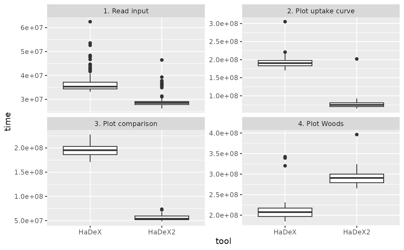
Figure 4.1: Benchmark results.
| task | HaDeX | HaDeX2 | Runtime ratio |
|---|---|---|---|
| 1. Read input | 34.83070 | 28.86460 | 0.8287115 |
| 2. Plot uptake curve | 171.86675 | 65.38155 | 0.3804200 |
| 3. Plot comparison | 186.86305 | 59.34140 | 0.3175663 |
| 4. Plot Woods | 201.53030 | 77.75905 | 0.3858430 |
| 5. Calculate confidence limit | 172.91570 | 53.16090 | 0.3074383 |
| 6. Reconstruct sequence | 24.18105 | 15.78765 | 0.6528935 |
Across all tasks, the reported values represent a runtime ratio (HaDeX2/HaDeX) consistently below one, indicating that HaDeX2 is faster than HaDeX for every measured operation. The strongest speedups, corresponding to the lowest ratios, are observed for plotting functions, calculating confidence limits, and plotting uptake curves, whereas input reading and sequence reconstruction show comparatively smaller, though still meaningful, reductions in execution time. In the case of input reading, the modest speed-up results from the fact that this functionality has substantially expanded in-built quality control in HaDeX2, where additional validation steps intentionally constrain maximal speed in favor of improved data integrity.
5 HaDeX2 design
The first version of HaDeX was developed quickly to address immediate data analysis challenges. As knowledge in the field expanded, it became necessary to extend the package’s functionality. This required a carefully planned redesign. The package is now built from small, modular computing blocks—encapsulated functions that each perform a single task. Datasets are created by combining these functions. This design allows individual components to be tested independently and improves code readability through self-explanatory function names (calculate_ provides results for specific time point, but create_dataset_ for all time points). The parameter naming conventions were also simplified. In addition, the graphical user interface was rewritten from scratch using Shiny modules to ensure clear separation and encapsulation of features.