Workflow description • HRaDeX

Article under development. This article covers in detail the classification workflow, alongside the numerical transformations. For the methods of visualization of results obtained using classification workflow, see the article on Visualization methods: vignette("visualization").

Introduction

The baseline of the HDX-MS method is the investigation of the exchange between hydrogen from the protein structure with deuterium from the buffer in which the protein is suspended. The difference in mass between hydrogen and deuterium is very close to 1 Da, so that we can identify the mass uptake with the number of exchanged hydrogens. Multiple time measurements allow us to see the exchange in time and create an exchange curve of the process for each measured and identified peptide (in a bottom-up approach).

The main challenge in HDX-MS is data analysis and interpretation. Although different methods of analysis focus on numerical values, that may be difficult to interpret, we wanted to propose a classification method to simplify communication of the results. Moreover, we are avoiding any data transformation, instead, propose a class label for perfectly known and valid experimental curves.

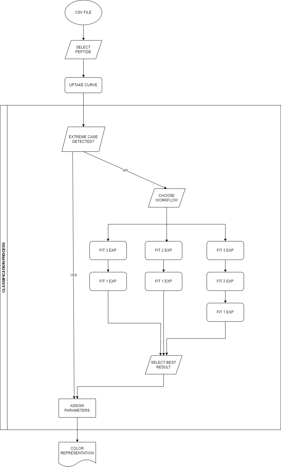
Classification method

This method aims to assign each peptide a specific combination of exchange classes, consistent with experimental results. This allows us to distinguish areas with different exchange patterns in the protein sequence, and to describe the exchange process itself.

The class assignment is the final step of the classification process, based on the literature description of the hydrogen-deuterium phenomenon. The process has several steps, with multiple workflow decisions under the experimenter’s control.

In the figure x, examples of experimental curves are presented. Although it is easy to discriminate between the extreme cases (described and defined in section x) - immediate exchange (red) and none-exchange (black), we need a classification method to provide information on the remaining curves (grey). The problem of classification is mainly focused on them.

Future plans: the classification of the subfragments of the overlapping peptides.

Obtaining the uptake curve

The experimental data from the csv file is processed and aggregated.
Firstly, the deuterium uptake curve is prepared. It is a function of deuterium uptake in time, with values defined as:

$D_t = m_t - m_0$

where $D_t$ is deuterium uptake in time $t$ in daltons, $m_t$ is mass of the peptide measured in time $t$ and $m_0$ is mass of undeuterated peptide.

Then, the uptake curve is normalized. The values are scaled according to the assumption, that the last time point of measurement or supplied fully deuterated control (difference explained below) is the maximal experimental deuterium uptake with 100% deuterium uptake. This can be calculated in two ways:

$D_{t, sc} = \frac{D_t}{D_{100}} = \frac{m_t - m_0}{m_{100} - m_0}$

This form of the uptake curve is used for the fitting process. Because of this, we can operate using percentages for populations (denoted as $n_i$ , the fraction of exchangeable hydrogens) undergoing different exchange patterns, and disregard the back-exchange problem for a while.

Comment on the difference between treating the last time point of measurement as fully deuterated (FD) control and additionally prepared fully deuteration control. When the first option is chosen, the last time point of measurement measuremnt ia assigned the value of 100% of deuterium uptake and the measurement point is taking part in the fitting process. When the additional fully deuterated control is chosen, all the measurement values are scaled with respect to that, but this FD value is not assigned to any time point, and not taking part in the fitting process, only the real measurement time points.

Extreme case recognition

Firstly, we recognize extreme cases of uptake curve, and assigned them a class name without fitting process.

For the peptide to be labeled as none exchange, has to fulfill defined requirements:

the uptake level [Da] in the last time point of measurement ( $D_{100}$ ) is lower than 1 Da,
the thoretical deuterium uptake in the last time point of measurement (scaled with respect to maximal possible uptake calculated from the sequence) is lower than 10%.

We interpret this case as a lack of observable exchange during the course of experiment, and indicate it with the black color on the visualization.

For the peptide to be disqualified from the fitting process and labeled by invalid there has to be lack of sufficient number of time points. It is crucial for the peptide to have valid measurements for $t_0$ and $t_100$ , as otherwise it prevents the normalization of values and causes the falsyfication of data. The missing of one or two time points of measurement (apart from controls) causes the use of two- or one- component model, but does not prevent the fitting process.

The fitting process is not conducted for uptake curves classified as extreme cases (no exchange or invalid).

Exchange class definition

Following the literature - especially in a cornerstone of the studies on the modeling hydrogen-deuterium exchange, the pioneering article of Zhang and Smith , we expect the process of deuterium exchange for the peptide to be described as a three-component equation x}:

$D = n_1 \cdot (1 - exp(-k_1 \cdot t)) + n_2 \cdot (1-exp(-k_2 \cdot t)) + n_3 \cdot (1 - exp(-k_3 \cdot t))$ where $n_i$ indicates the population of i-th group and $k_i$ is the exchange rate of i-th group. Moreover, we assume:

$n_1$ , $k_1$ - fast exchange (red)
$n_2$ , $k_2$ - medium exchange (green)
$n_3$ , $k_3$ - slow exchange (blue)

Ideally, $n_1 + n_2 + n_3 = 1$ . In this equation, we have six unknown parameters that need to be found.

Unfortunately, the authors of this paper did not provide boundaries for each exchange group. The ranges proposed by us, according to our experience, can be found in table x.

The ranges of exchange rates can be changed if desired. However, we recommend avoiding situations where a certain range is covered by two classes, as it may lead to misclassification.

	lower	upper
$k_1$	1	30
$k_2$	0.1	1
$k_3$	0	0.1

The Zhang & Smith equation describes a theoretical situation, which may not occur during every experiment. Thus, we prepared different workflows and modifications (described later on), but the three-component equation is our desired starting point.

Workflow selection

We have multiple workflows prepared. We strongly advise using the first one, but we understand the specificity of each experiment and we leave the final decision to the user, trusting their motives.

Available workflows:

3exp/1exp - we start the fitting process by looking for the best fit using function x with ranges specified in table x}. For the peptides with unsatisfactory results, we look for only one component function (described below). The selection of better results is made by comparing the $R^2$ values.
2exp/1exp - the starting point is the two-component function (described below), and then the one-component function. The decision process is the same as in the previous point.
3exp/2exp/1exp - all of the variants of the fitting process are prepared and the best is chosen based on the $BIC$ value.

3exp fit

The fitting function is described as Zhang & Smith equation x, with initial values:

$n_1 = n_2 = n_3 = 0.33$
$k_1 = 1$
$k_2 = 0.1$
$k_3 = 0.01$

The boundaries for the values are as described in table x.

The number of unknown parameters is 6.

2exp fit

The two-component fitting function, is described as follows:

$D = n_a \cdot (1 - exp(-k_a \cdot t)) + n_b \cdot (1-exp(-k_b \cdot t))$

Where $a$ and $b$ are two of three exchange groups defined for the Zhang & Smith equation. We perform three fitting processes (for each group combination) and select the best result comparing the $R^2$ value. That means we look for the fit using $k_1$ with $k_2$ , $k_2$ with $k_3$ , or $k_1$ with $k_3$ and select one as the answer.

The initial value for $n_a$ and $n_b$ is 0.5. The initial values for $k$ are the same with analogical cases from the three-component equation (see section x).

In this case, we assume that $n_a$ of hydrogen particles are undergoing the exchange with $k_a$ exchange rate, an $n_b$ with exchange rate $k_b$ .

The number of unknown parameters is 4.

1exp fit

The fitting function is described as follows:

$D = n \cdot (1 - exp(-k \cdot t))$

In this case, we assume that all of the hydrogen particles in the peptide are undergoing the exchange in a similar way. Ideally with $n \sim 1$ .

The initial values for the fit:

$n = 1$
$k = 1$
upper boundary of $k$ = upper boundary of $k_1$
lower boundary of $k$ = lower boundary of $k_3$

The number of unknown parameters is 2.

Fitting parameters

To fit the curve we use the nonlinear least square method. For more information, see the documentation of the used R package.

Recommended parameters (possible change):

max iteration: 100,
algorithm: Levenberg-Marquardt.

Results of the fitting process

TODO: n, k, rgb, interpretation

Calculation of estimed exchange rate k

As we are working on normalized values and each value $n_i$ is within the limits of (0, 1), whe can treat them somehow as a probability of getting $k_i$ . Then, we can caluclate the estimate k value, aggrgating all of the fit parameters into one value:

$k_{exp} = \sum^i n_i \cdot k_i$

High resolution results

As the classification is performed on uptake curves of each peptide, there is a need of aggrgation to obtain the high resolution results. Currently, HRaDeX allows the use of two methods.

Selection of the shortest peptide.

For each residue there is a subset of peptides covering said residue. From this set, the shortest peptide is chosen as a determinant for the resiude, as the most represantative.

Aggregation of values

Aggregation of values is inspired by the article by Keppler and Weis (doi: 10.1007/s13361-014-1033-6), with small changes: the ommition of the first residue is done in different step if demanded by the user. The aggregation of values is done on a subset of already filtered data.

For each residue there is a subset of peptides covering said residue. Then, the final $n_{i, agg}$ is calculated from the subset of $n_i$ , with weights inverse proportional to the max uptake of peptide ( $mu_i$ ) - the shortest the peptide the highest the possibility that the uptake took place in said residue:

$w_i = \frac{\frac{1}{mu_i}}{\sum^i \frac{1}{mu_i}}$

Then, the $n_i%$ is a weighted average of set of $n_i$ .

$n_{i, agg} = \frac{\sum^i w_i \cdot n_i}{\sum^i w_i}$ There is a possibility that $n_{i, agg}$ obtained that way exceeds the limit of 1. Then, we normalize the values, to get the sense of proportionality.

$n_{i, agg.scaled} = \frac{n_{i, agg}}{\sum^i n_{i, agg}}$

This way, we have the right values to obtain the RGB color value.

The estimated k values are calculated analogically.

Workflow schema

Figure x presents the diagram for classifying one peptide in one biological state, based on its uptake curve. This process can be repeated for each peptide from the data file to access the information for the set of peptides from a protein.

Workflow schema